

Algorithm Research Based on the PDE Sensitivity Filter
-
摘要:
采用PDE灵敏度滤波器可以消除连续体结构拓扑优化结果存在的棋盘格现象、数值不稳定等问题,且PDE灵敏度滤波器的实质是具有Neumann边界条件的Helmholtz偏微分方程。针对大规模PDE灵敏度滤波器的求解问题,有限元分析得到其代数方程,分别采用共轭梯度算法、多重网格算法和多重网格预处理共轭梯度算法对代数方程进行求解,并且研究精度、过滤半径以及网格数量对拓扑优化效率的影响。结果表明:与共轭梯度算法和多重网格算法相比,多重网格预处理共轭梯度算法迭代次数最少,运行时间最短,极大地提高了拓扑优化效率。
-
关键词:
- PDE滤波器 /
- Helmholtz方程 /
- 多重网格算法 /
- 共轭梯度算法 /
- 拓扑优化
Abstract:The PDE sensitivity filter can eliminate the checkerboard patterns and numerical instability existing in the topology optimization results of continuum structures, and the essence of the PDE sensitivity filter is the Helmholtz partial differential equation with Neumann boundary conditions. To solve the large-scale PDE sensitivity filter problem, the conjugate gradient algorithm, the multigrid algorithm and the multigrid preconditioned conjugate gradient algorithm were used to solve the algebraic equations obtained by finite element analysis, and the effects of accuracy, filter radius and grid numbers on the efficiency of topology optimization were studied. The results show that, compared with the conjugate gradient algorithm and the multi-grid algorithm, the multi-grid preconditioned conjugate gradient algorithm has the least number of iterations and the shortest running time, which greatly improves the efficiency of topology optimization.
-
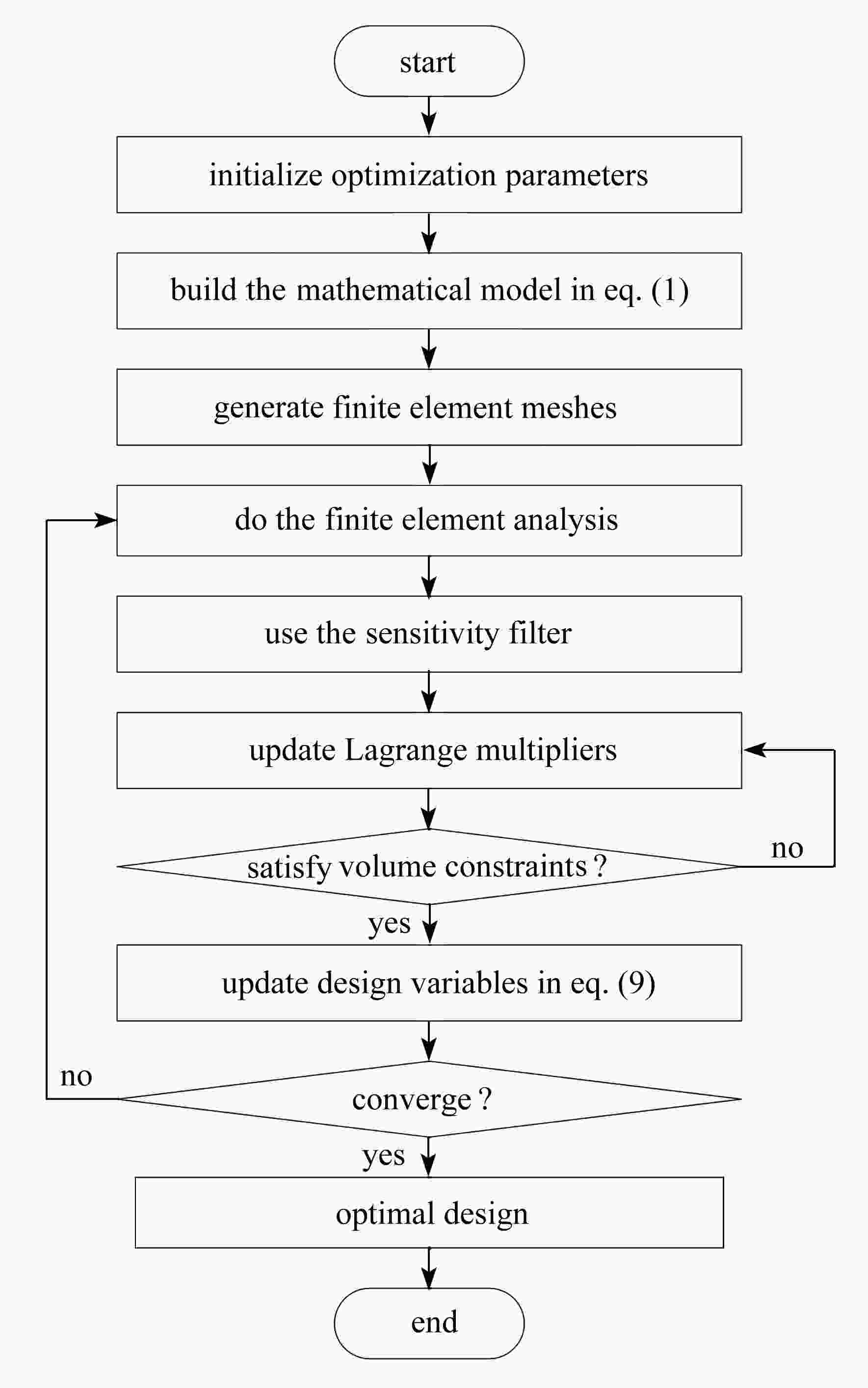
图 1 基于SIMP插值模型连续体结构拓扑优化实现流程图
Figure 1. The flow chart of continuum structure topology optimization based on the SIMP interpolation model
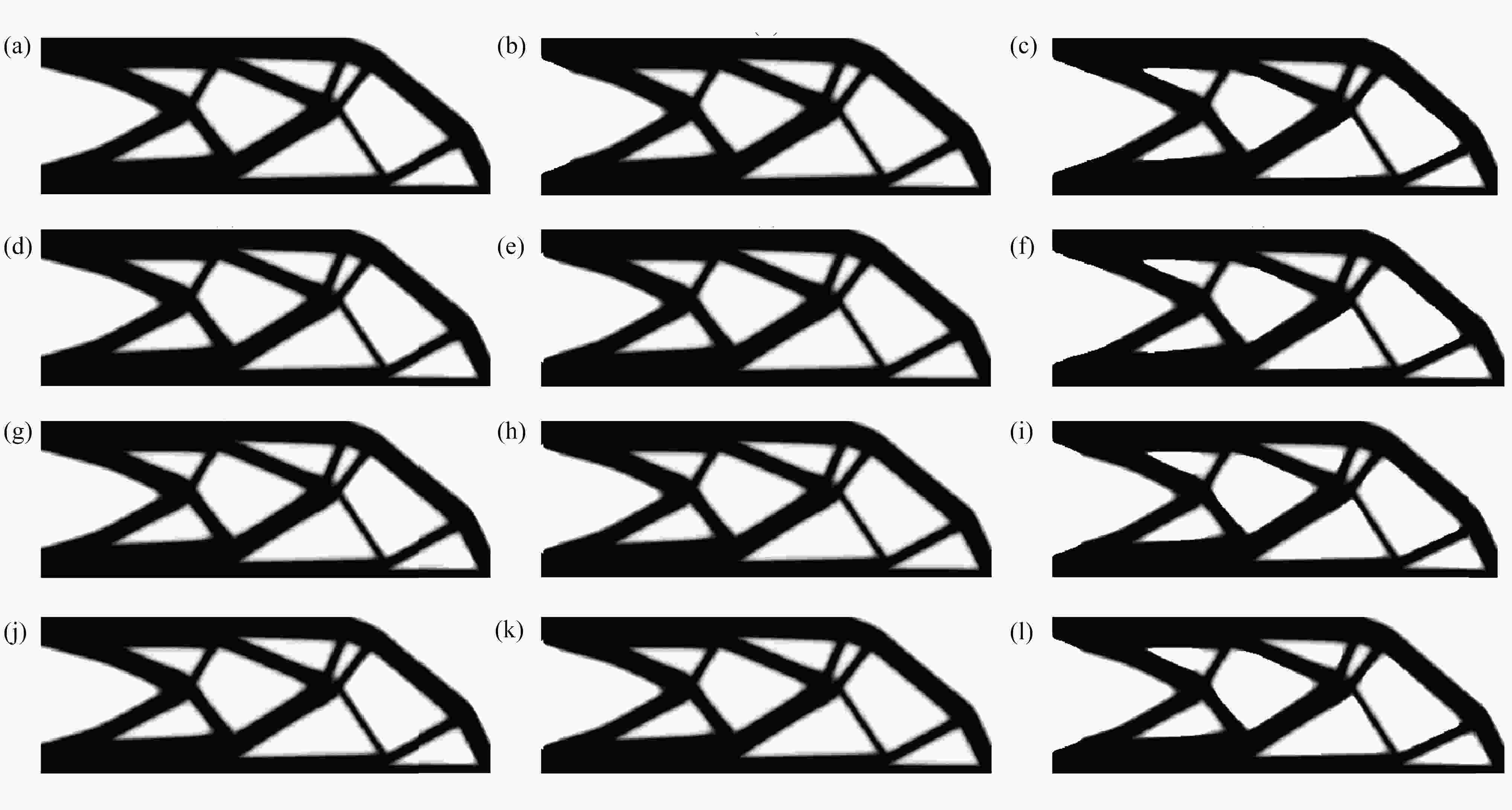
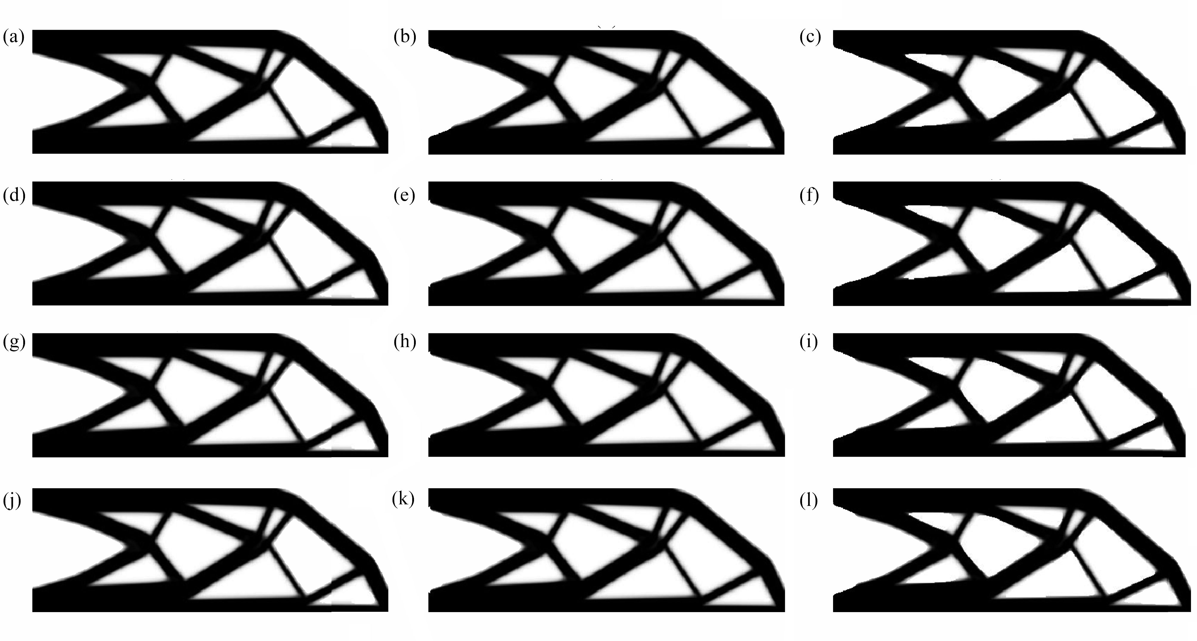
图 4 不同精度下CG、MG和MGCG算法的悬臂梁的优化结构:(a) P=1E−2 (CG);(b) P=1E−2 (MG);(c) P=1E−2 (MGCG);(d) P=1E−3 (CG);(e) P=1E−3 (MG);(f) P=1E−3 (MGCG);(g) P=1E−4 (CG);(h) P=1E−4 (MG);(i) P=1E−4 (MGCG);(j) P=1E−5 (CG);(k) P=1E−5 (MG);(l) P=1E−5 (MGCG)
Figure 4. The optimized cantilever beams by CG, MG and MGCG algorithms with different degrees of precision: (a) P=1E−2 (CG); (b) P=1E−2 (MG); (c) P=1E−2 (MGCG); (d) P=1E−3 (CG); (e) P=1E−3 (MG); (f) P=1E−3 (MGCG); (g) P=1E−4 (CG); (h) P=1E−4 (MG); (i) P=1E−4 (MGCG); (j) P=1E−5 (CG); (k) P=1E−5 (MG); (l) P=1E−5 (MGCG)
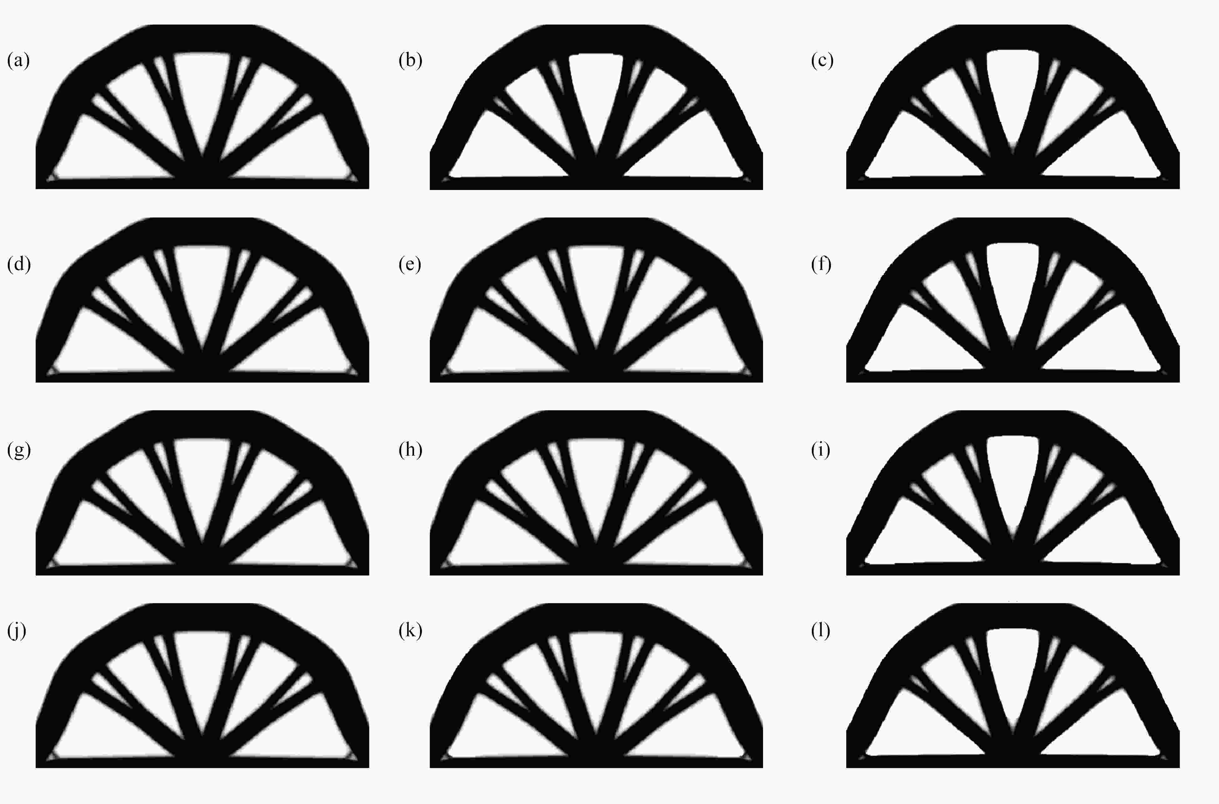
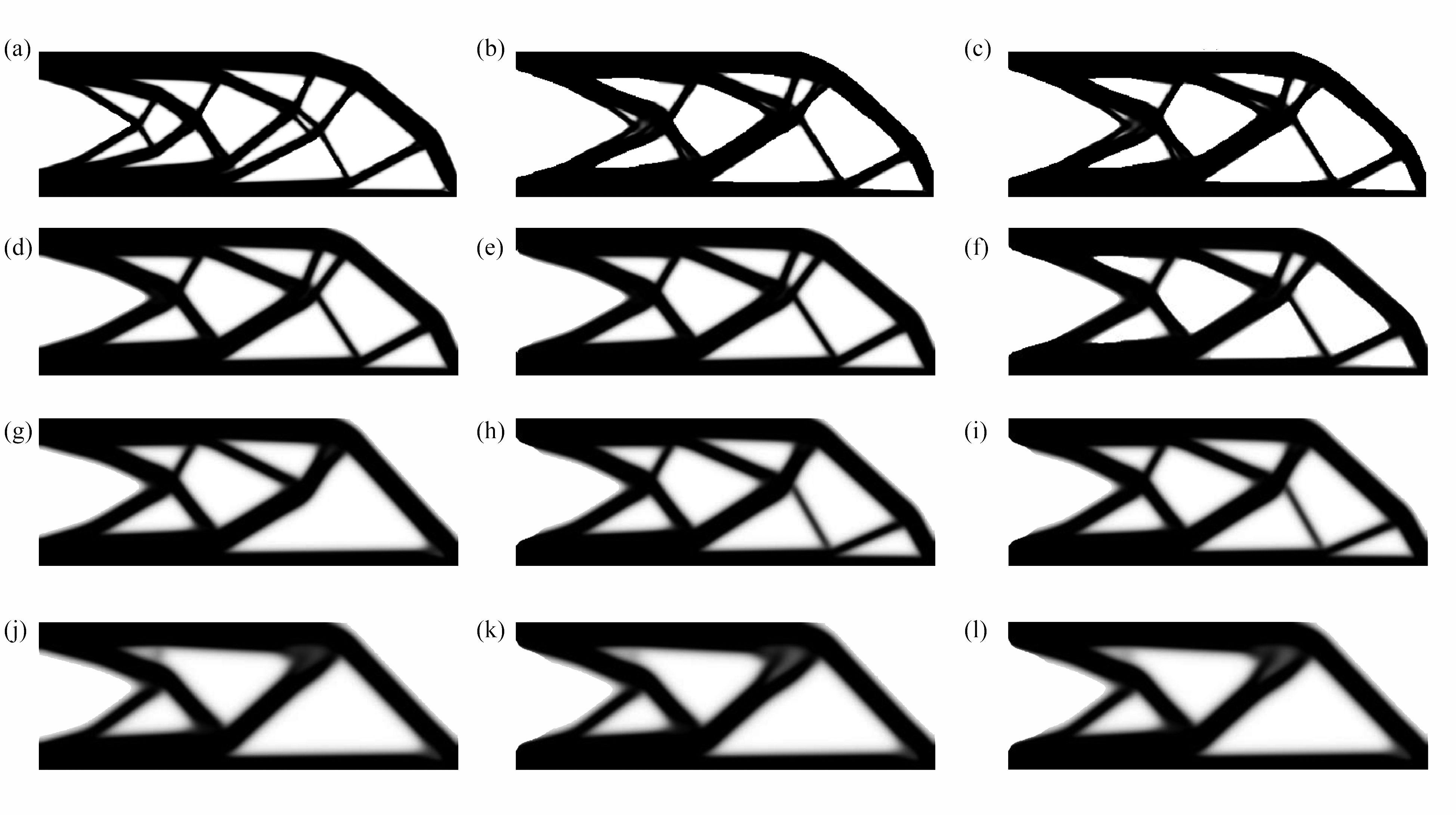
图 5 不同精度下CG、MG和MGCG算法的Michell结构的优化结构:(a) P=1E−2 (CG);(b) P=1E−2 (MG);(c) P=1E−2 (MGCG);(d) P=1E−3 (CG);(e) P=1E−3 (MG);(f) P=1E−3 (MGCG);(g) P=1E−4 (CG);(h) P=1E−4 (MG);(i) P=1E−4 (MGCG);(j) P=1E−5 (CG);(k) P=1E−5 (MG); (l) P=1E−5 (MGCG)
Figure 5. The optimized Michell structures by CG, MG and MGCG algorithms with different degrees of precision: (a) P=1E−2 (CG); (b) P=1E−2 (MG); (c) P=1E−2 (MGCG); (d) P=1E−3 (CG); (e) P=1E−3 (MG); (f) P=1E−3 (MGCG); (g) P=1E−4 (CG); (h) P=1E−4 (MG); (i) P=1E−4 (MGCG); (j) P=1E−5 (CG); (k) P=1E−5 (MG); (l) P=1E−5 (MGCG)
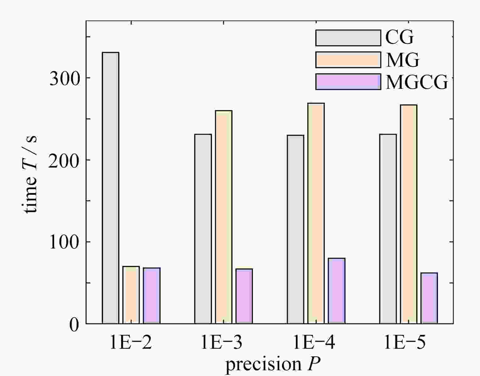
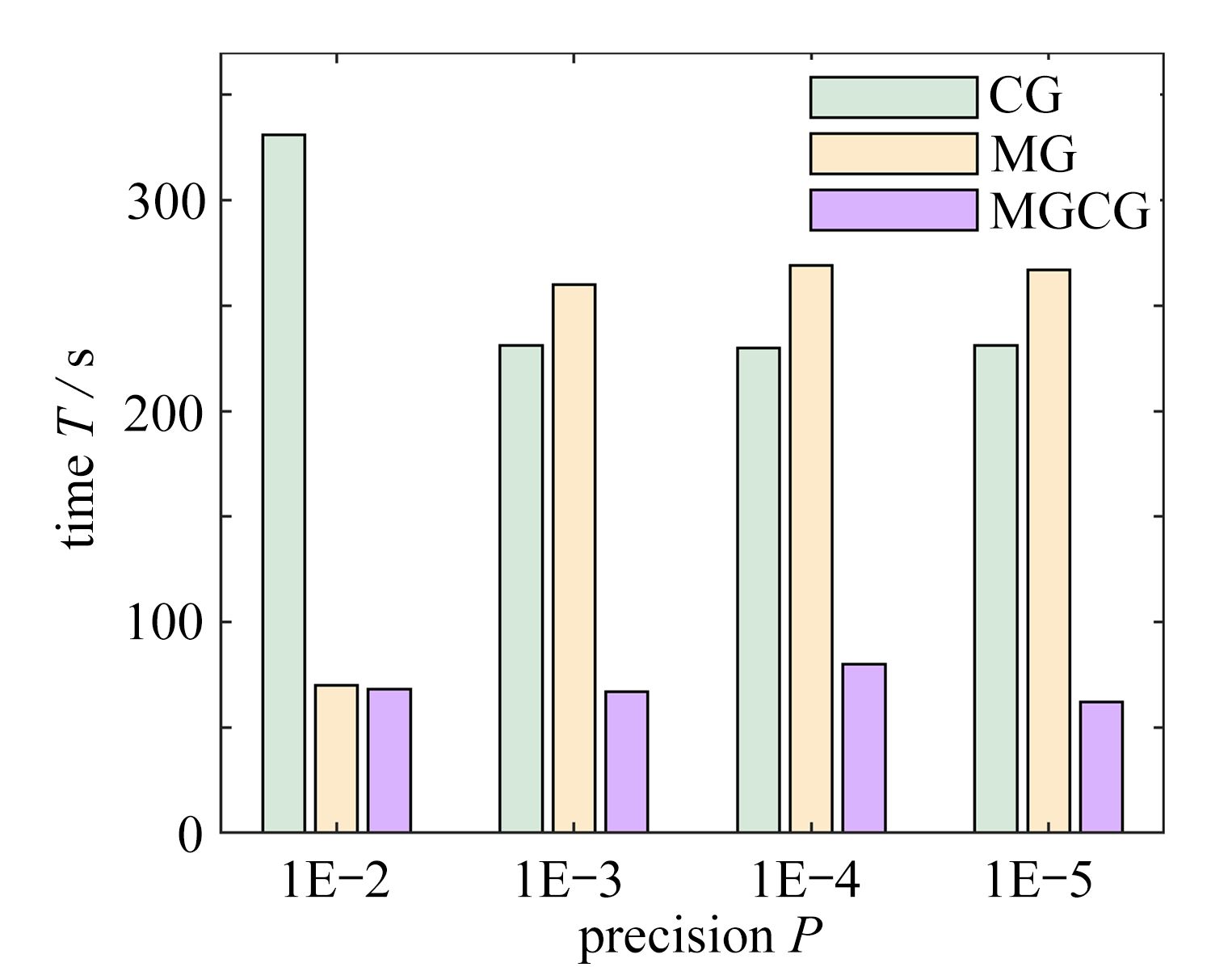
图 7 Michell结构优化时间分布图
Figure 7. The optimized time distribution of the Michell structure
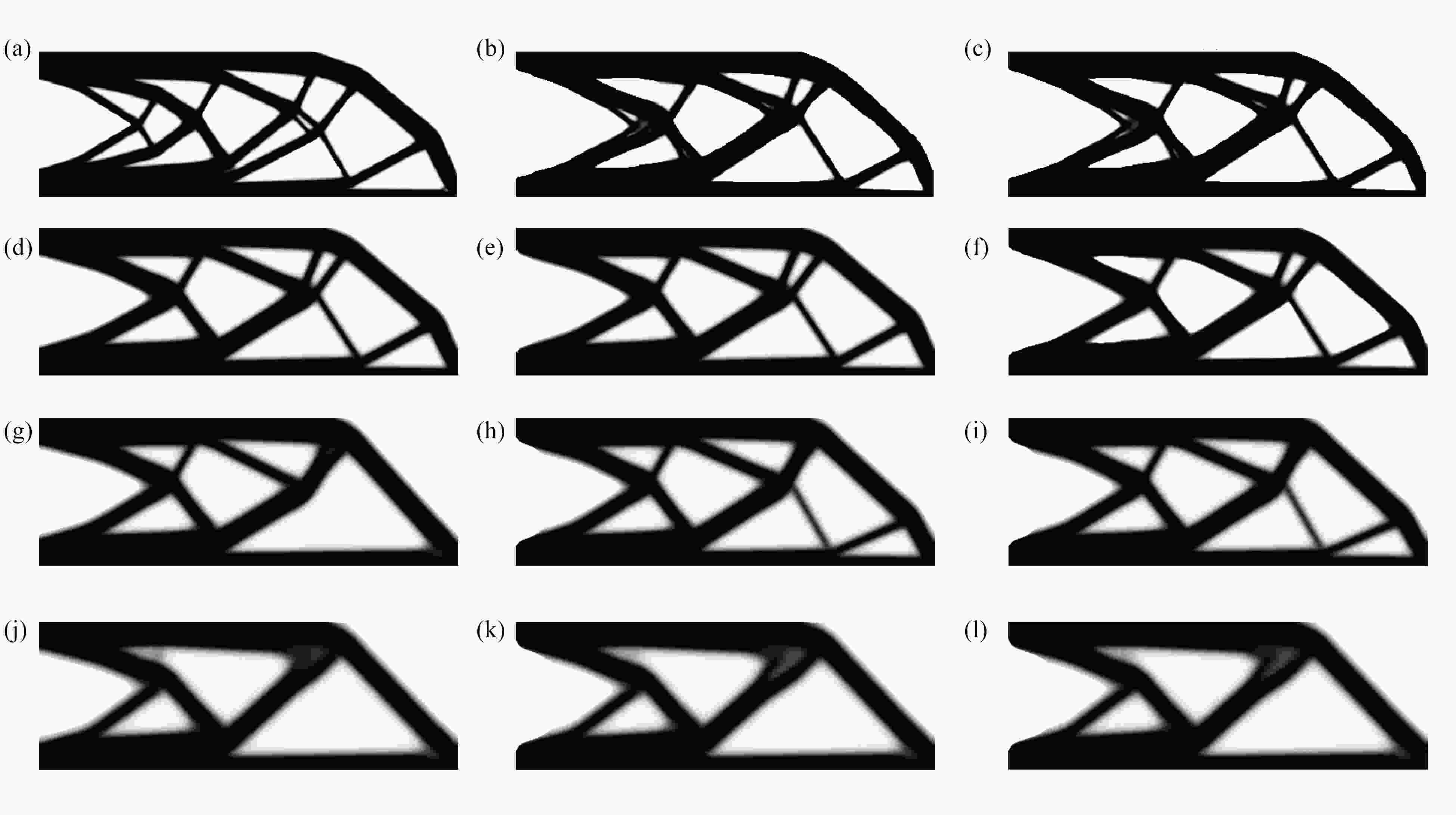
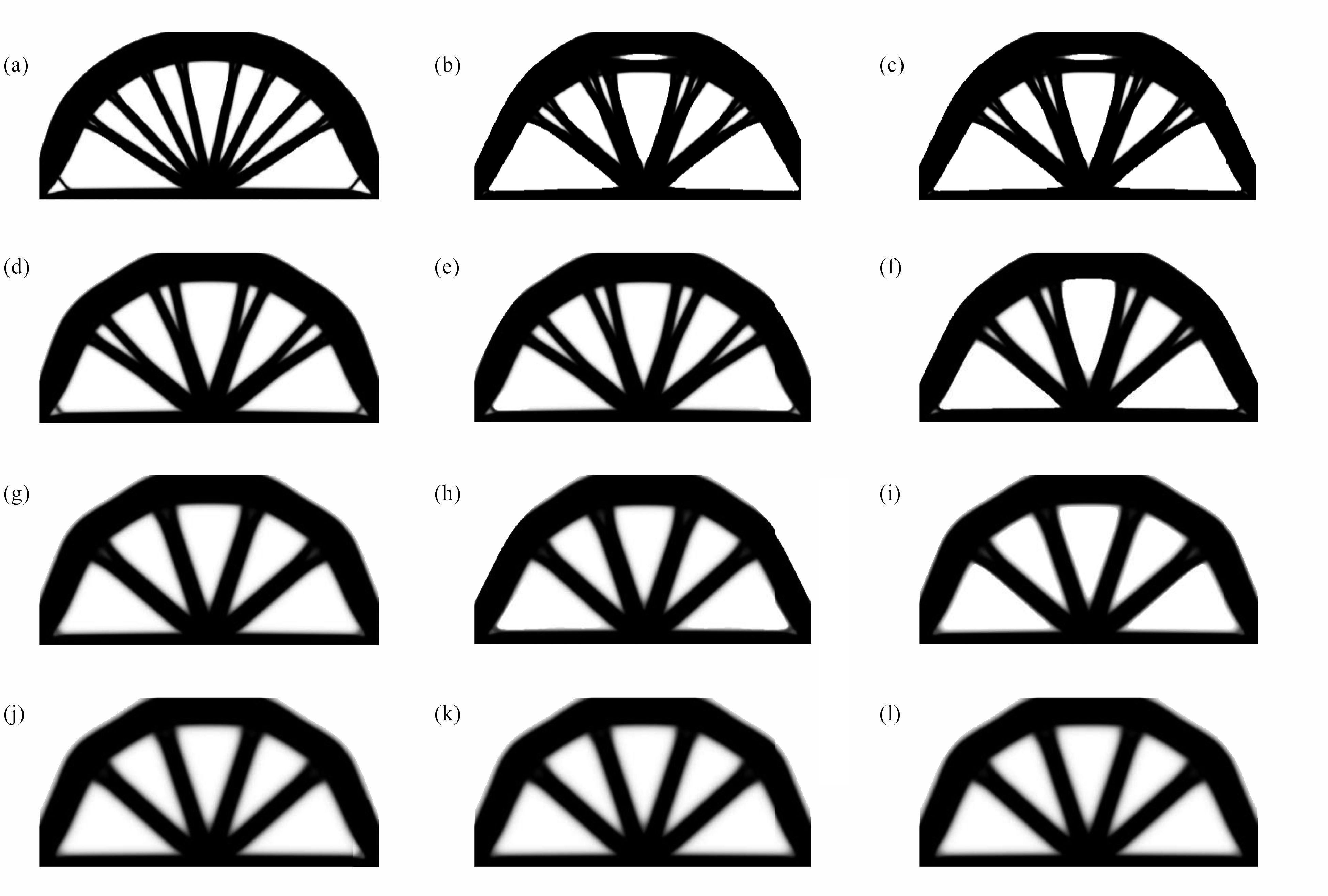
图 8 不同过滤半径下CG、MG和MGCG算法的悬臂梁的优化结构:(a) R=3 (CG);(b) R=3 (MG);(c) R=3 (MGCG);(d) R=6 (CG);(e) R=6 (MG);(f) R=6 (MGCG);(g) R=9 (CG);(h) R=9 (MG);(i) R=9 (MGCG);(j) R=12 (CG);(k) R=12 (MG);(l) R=12 (MGCG)
Figure 8. The optimized cantilever beams by CG, MG and MGCG algorithms with different filter radius: (a) R=3 (CG); (b) R=3 (MG); (c) R=3 (MGCG); (d) R=6 (CG); (e) R=6 (MG); (f) R=6 (MGCG); (g) R=9 (CG); (h) R=9 (MG); (i) R=9 (MGCG); (j) R=12 (CG); (k) R=12 (MG); (l) R=12 (MGCG)
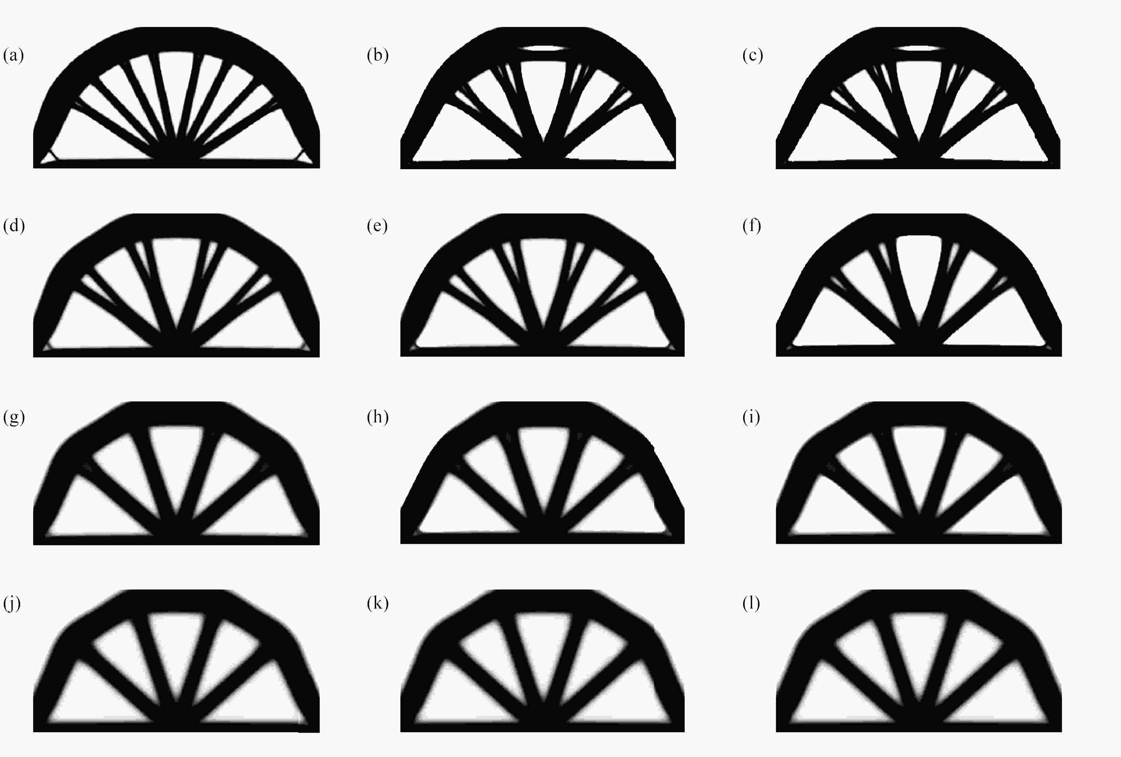
图 9 不同过滤半径下CG、MG和MGCG算法的Michell结构的优化结构:(a) R=3 (CG);(b) R=3 (MG);(c) R=3 (MGCG);(d) R=6 (CG);(e) R=6 (MG);(f) R=6 (MGCG);(g) R=9 (CG);(h) R=9 (MG);(i) R=9 (MGCG);(j) R=12 (CG);(k) R=12 (MG);(l) R=12 (MGCG)
Figure 9. The optimized Michell structures by CG, MG and MGCG algorithms with different filter radius: (a) R=3 (CG); (b) R=3 (MG); (c) R=3 (MGCG); (d) R=6 (CG); (e) R=6 (MG); (f) R=6 (MGCG); (g) R=9 (CG); (h) R=9 (MG); (i) R=9 (MGCG); (j) R=12 (CG); (k) R=12 (MG); (l) R=12 (MGCG)

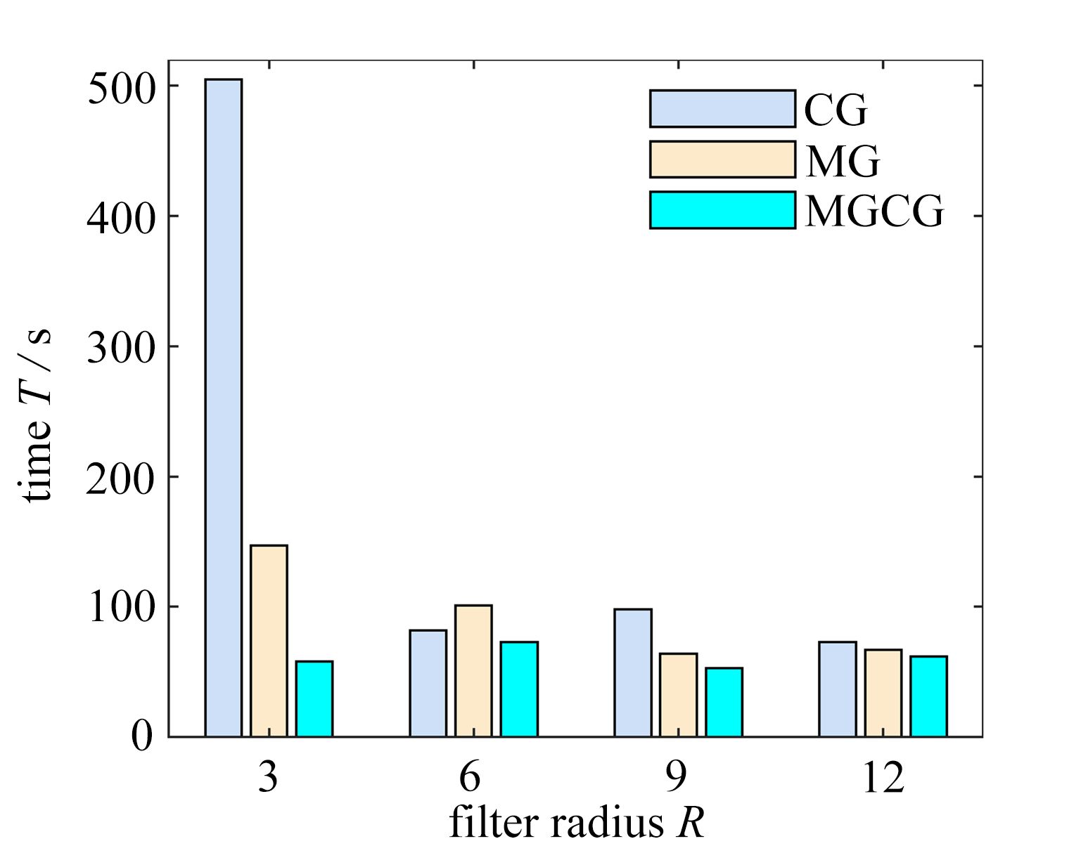
图 10 悬臂梁结构优化时间分布图(不同过滤半径)
Figure 10. The optimized time distribution of the cantilever beam (different filter radius)
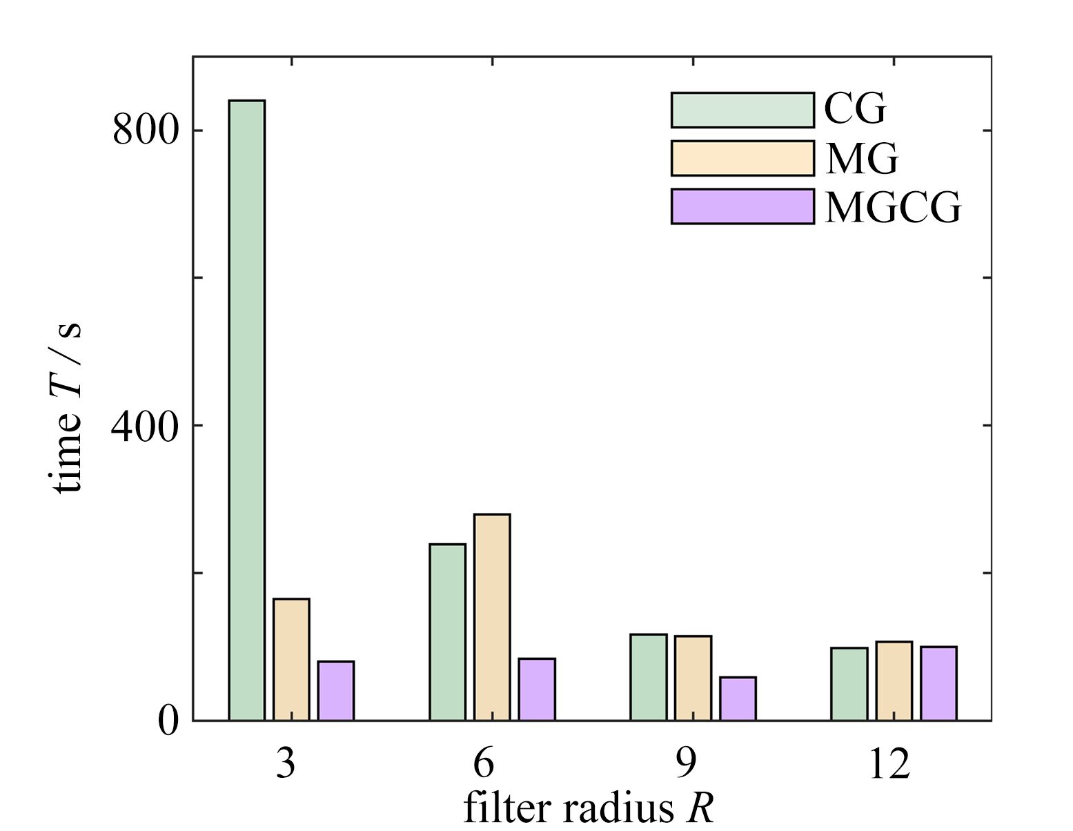
图 11 Michell结构优化时间分布图(不同过滤半径)
Figure 11. The optimized time distribution of the Michell structure (different filter radius)
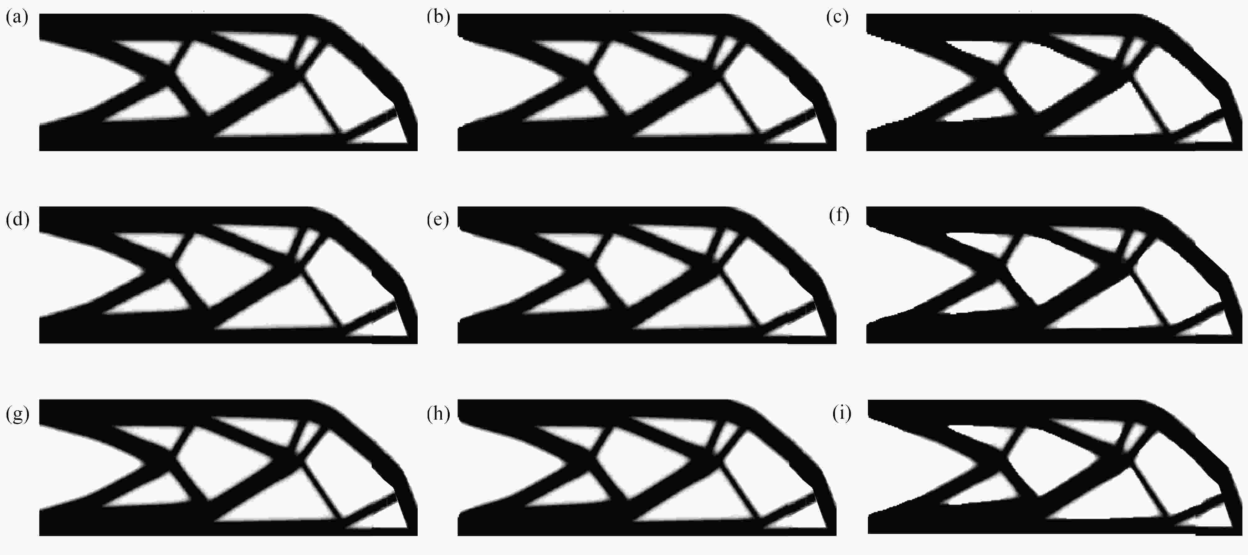
图 12 不同网格数量下CG、MG和MGCG算法的悬臂梁的优化结构:(a) 网格为240 × 80 (CG);(b) 网格为240 × 80 (MG);(c) 网格为240 × 80 (MGCG);(d) 网格为480 × 160 (CG);(e) 网格为480 × 160 (MG);(f) 网格为480 × 160 (MGCG);(g) 网格为960 × 320 (CG);(h) 网格为960 × 320 (MG);(i) 网格为960 × 320 (MGCG)
Figure 12. The optimized cantilever beams by CG, MG and MGCG algorithms with different grids: (a) grid 240 × 80 (CG); (b) grid 240 × 80 (MG); (c) grid 240 × 80 (MGCG); (d) grid 480 × 160 (CG); (e) grid 480 × 160 (MG); (f) grid 480 × 160 (MGCG); (g) grid 960 × 320 (CG); (h) grid 960 × 320 (MG); (i) grid 960 × 320 (MGCG)
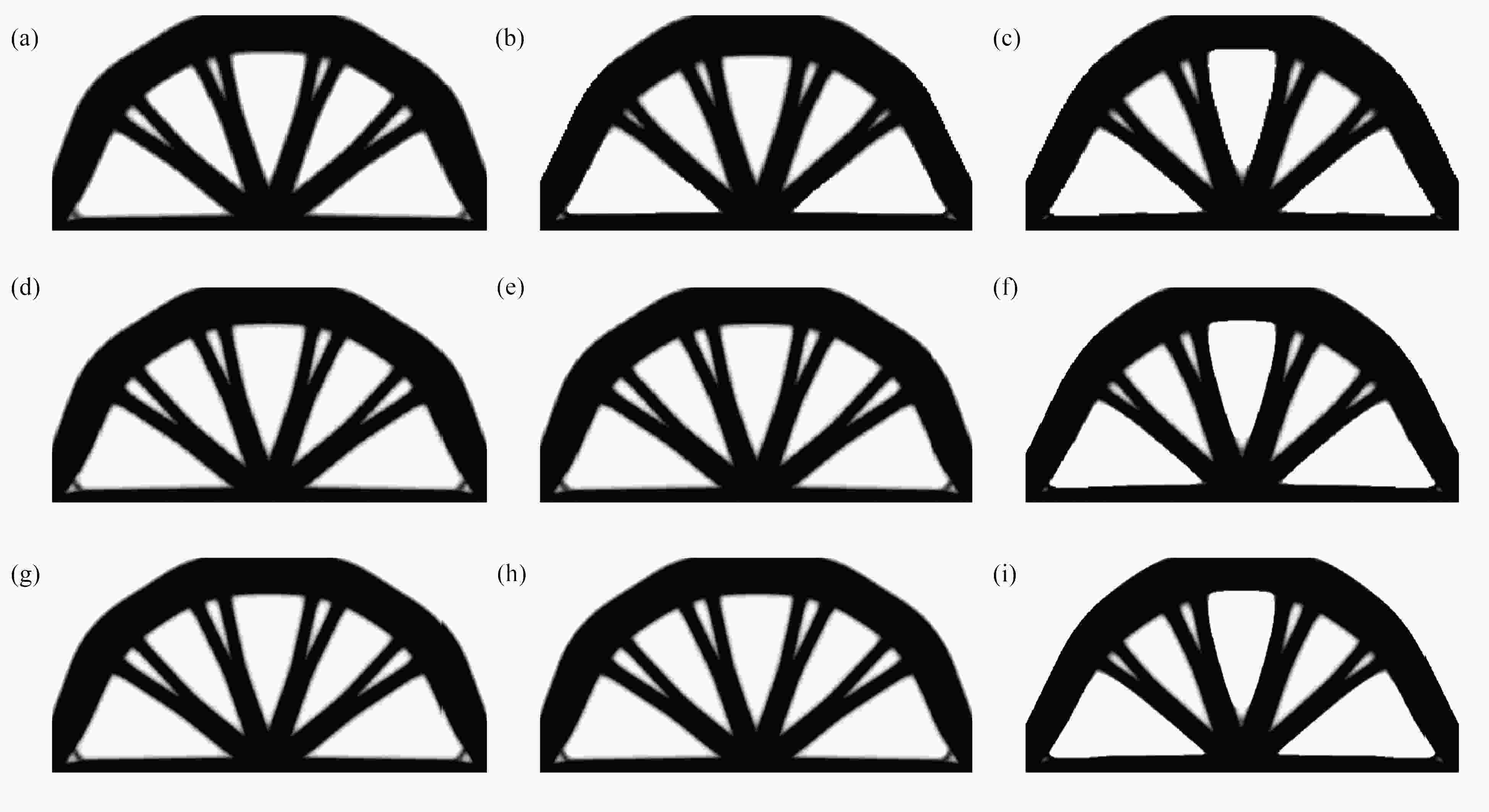
图 13 不同网格数量下CG、MG和MGCG算法的Michell结构的优化结构:(a) 网格为240 × 120 (CG);(b) 网格为240 × 120 (MG);(c) 网格为240 × 120 (MGCG);(d) 网格为480 × 240 (CG);(e) 网格为480 × 240 (MG);(f) 网格为480 × 240 (MGCG);(g) 网格为960 × 480 (CG);(h) 网格为960 × 480 (MG);(i) 网格为960 × 480 (MGCG)
Figure 13. The optimized Michell structures by CG, MG and MGCG algorithms with different grids: (a) grid 240 × 120 (CG); (b) grid 240 × 120 (MG); (c) grid 240 × 120 (MGCG); (d) grid 480 × 240 (CG); (e) grid 480 × 240 (MG); (f) grid 480 × 240 (MGCG); (g) grid 960 × 480 (CG); (h) grid 960 × 480 (MG); (i) grid 960 × 480 (MGCG)

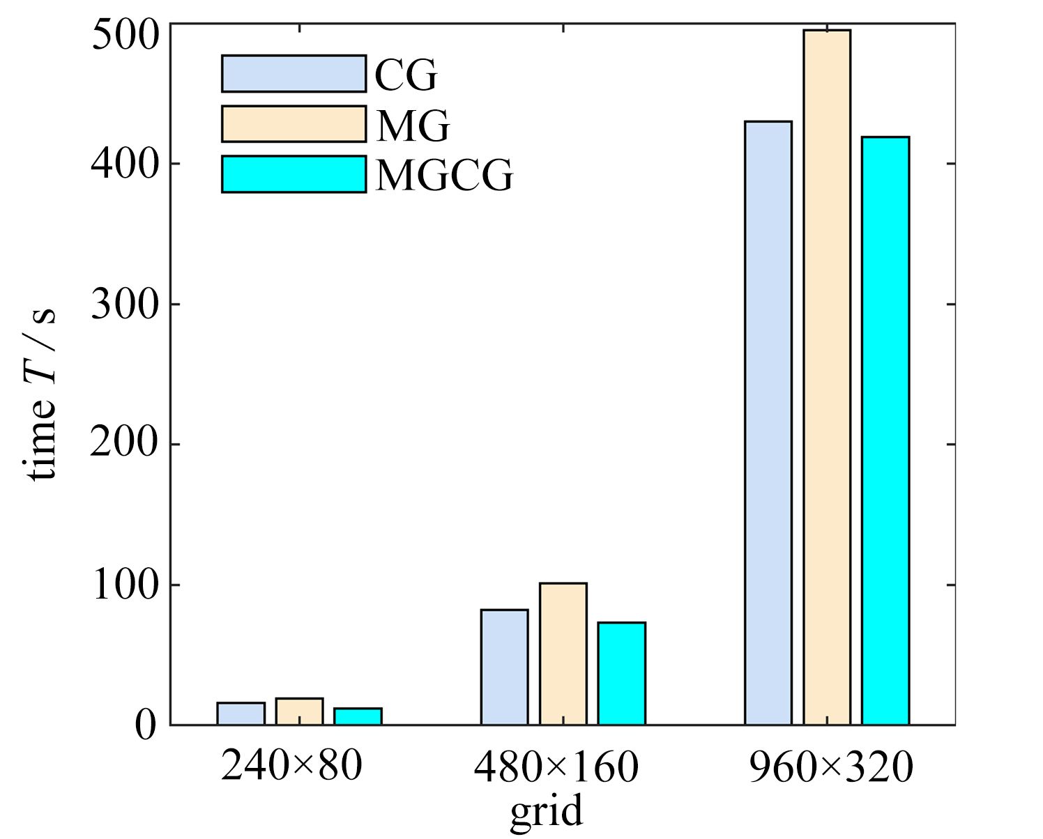
图 14 悬臂梁结构优化时间分布图(不同网格数量)
Figure 14. The optimized time distribution of the cantilever beam (different grids)
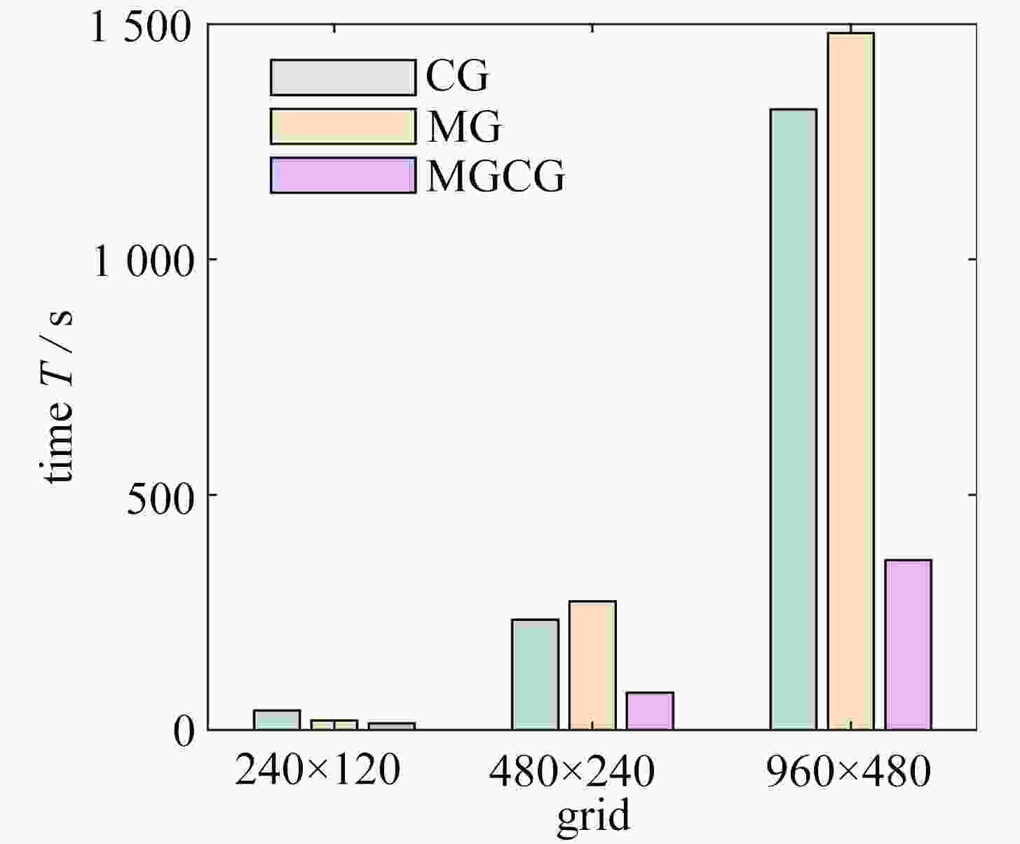
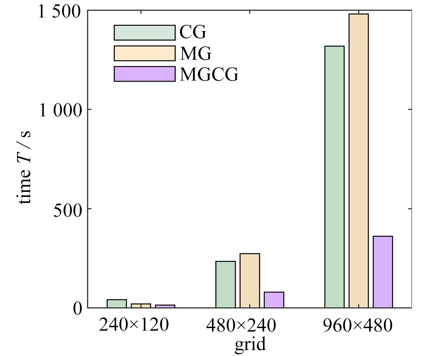
图 15 Michell结构优化时间分布图(不同网格数量)
Figure 15. The optimized time distribution of the Michell structure (different grids)
算法1 1 input: 2 level k; 3 initial guess $ {\boldsymbol{u}}_k^m $; 4 right hand side vector $ {{\boldsymbol{f}}_k} $; 5 coefficient matrix under level $ k $ grid $ {{\boldsymbol{A}}_k} $; 6 output: 7 updated solution $ {\boldsymbol{u}}_k^{m + 1} $ 8 pre-smooth: $ {\boldsymbol{u}}_k^{m + 1} = {{\boldsymbol{S}}^{{\mu _1}}}({{\boldsymbol{A}}_k},{{\boldsymbol{f}}_k},{\boldsymbol{u}}_k^m) $ 9 coarse grid correction: 10 compute residual: $ {\boldsymbol{r}}_k^m = {{\boldsymbol{f}}_k} - {{\boldsymbol{A}}_k}{\boldsymbol{u}}_k^m $ 11 restrict the residual to coarse-grid: $ {\boldsymbol{r}}_{k + 1}^m = {\boldsymbol{R}}_k^{k + 1}{\boldsymbol{r}}_k^m $ 12 if k + 1=L then 13 solve approximate error solution $ \tilde {\boldsymbol{e}}_{k + 1}^m = {\boldsymbol{A}}_{k + 1}^{ - 1}{\boldsymbol{r}}_{k + 1}^m $ 14 else 15 $ \tilde {\boldsymbol{e}}_{k + 1}^m{\text{ = }}V \cdot {\text{cycle(}}{{\boldsymbol{A}}_{k + 1}},{\boldsymbol{r}}_{k + 1}^m,0,k + 1) $ 16 end 17 interpolate: 18 $ \tilde {\boldsymbol{e}}_k^m = P_{k + 1}^k\tilde {\boldsymbol{e}}_{k + 1}^m $ 19 $ {\boldsymbol{u}}_k^{m + 1} = {\boldsymbol{u}}_k^{m + 1} + \tilde {\boldsymbol{e}}_k^m $ 20 post-smooth: 21 $ {\boldsymbol{u}}_k^{m + 1} = {{\boldsymbol{S}}^{{\mu _2}}}({{\boldsymbol{A}}_k},{{\boldsymbol{f}}_k},{\boldsymbol{u}}_k^{m + 1}) $。  下载: 导出CSV
算法2 input: symmetric positive definite coefficient matrix $ {\boldsymbol{A}} $; right hand side vector $ {\boldsymbol{b}} $; initiate a guess for $ {{\boldsymbol{x}}_0} \in {\mathbb{R}^n} $ output: solution $ {\boldsymbol{x}} $; 1 compute the residual on the finest grid $ {{\boldsymbol{r}}_0} \mathop {\rm{ = }}\limits^\Delta {\boldsymbol{b}} - {\boldsymbol{A}}{{\boldsymbol{x}}_0} $; 2 for $ i = 1,2,3, \cdots $ do 3 solve $ {\boldsymbol{A}}{{\boldsymbol{z}}_0} = {{\boldsymbol{r}}_0} $ by the multigrid V-cycle algorithm 4 initialize $ {{\boldsymbol{p}}_0} = {{\boldsymbol{z}}_0} $ 5 compute a step length the $ {\alpha _i} = ({\boldsymbol{r}}_{i - 1}^{\text{T}}{{\boldsymbol{z}}_{i - 1}})/({\boldsymbol{p}}_{i - 1}^{\text{T}}{\boldsymbol{A}}{{\boldsymbol{p}}_{i - 1}}) $ (where $ {{\boldsymbol{z}}_{i - 1}} $ can be solved by the multigrid V-cycle algorithm) 6 update the approximate solution $ {{\boldsymbol{x}}_i} = {{\boldsymbol{x}}_{i - 1}} + {\alpha _i}{{\boldsymbol{p}}_{i - 1}} $ 7 update the residual $ {{\boldsymbol{r}}_i} = {{\boldsymbol{r}}_{i - 1}} - {\alpha _i}{\boldsymbol{A}}{{\boldsymbol{p}}_{i - 1}} $ 8 solve $ {\boldsymbol{A}}{{\boldsymbol{z}}_i} = {{\boldsymbol{r}}_i} $ by the multigrid V-cycle algorithm 9 compute a gradient correction factor $ {\beta _i} = ({\boldsymbol{r}}_i^{\rm{T}}{{\boldsymbol{z}}_i})/({\boldsymbol{r}}_{i - 1}^{\rm{T}}{{\boldsymbol{z}}_{i - 1}}) $ 10 set the new search direction $ {{\boldsymbol{p}}_i} = {{\boldsymbol{z}}_i} + {\beta _i}{{\boldsymbol{p}}_{i - 1}} $ 11 end 12 until convergence。
下载: 导出CSV
表 1 两种结构的拓扑优化迭代次数和柔度值
Table 1. Total numbers of iterations and compliance for topology optimization of 2 structures
structure precision P CG algorithm MG algorithm MGCG algorithm compliance C time T/s iterations I compliance C time T/s iterations I compliance C time T/s iterations I cantilever beam 1E−2 186.885 2 87 170 187.306 9 96 167 184.738 3 64 114 1E−3 186.883 4 82 155 186.939 3 100 160 184.414 7 54 100 1E−4 186.884 2 84 155 186.939 2 105 160 184.014 0 75 133 1E−5 186.883 9 84 155 186.939 1 111 160 185.215 5 64 113 Michell structure 1E−2 17.125 2 331 387 16.909 5 70 78 16.923 8 68 78 1E−3 17.123 4 231 271 17.119 9 260 277 16.923 9 67 78 1E−4 17.123 1 230 271 17.119 9 269 277 16.952 6 80 93 1E−5 17.123 1 231 271 17.074 7 267 267 16.943 6 62 71
下载: 导出CSV
表 2 两种结构的拓扑优化迭代次数和柔度值(不同过滤半径)
Table 2. Total numbers of iterations and compliance for topology optimization of 2 structures (different filter radius)
structure filter radius R CG algorithm MG algorithm MGCG algorithm compliance C time T/s iterations I compliance C time T/s iterations I compliance C time T/s iterations I cantilever beam 3 180.759 1 505 917 182.218 3 147 225 182.352 0 58 103 6 186.884 2 82 155 186.939 2 101 160 184.014 0 73 133 9 192.522 9 98 183 193.053 7 64 100 193.096 7 53 97 12 197.418 7 73 136 197.669 5 67 105 197.641 9 62 115 Michell structure 3 16.738 5 840 926 16.864 5 165 168 16.894 1 80 90 6 17.123 1 239 271 17.119 9 280 277 16.952 6 84 93 9 17.382 9 117 133 17.322 6 115 117 17.168 6 59 67 12 17.696 4 99 114 17.696 5 107 114 17.686 4 100 114
下载: 导出CSV
表 3 两种结构的拓扑优化迭代次数和柔度值(不同网格数量)
Table 3. Total numbers of iterations and compliance for topology optimization of 2 structures (different grids)
structure grid size CG algorithm MG algorithm MGCG algorithm compliance C time T/s iterations I compliance C time T/s iterations I compliance C time T/s iterations I cantilever beam 240 × 80 186.484 0 16 133 186.315 3 19 133 183.148 4 12 96 480 × 160 186.884 2 82 155 186.939 2 101 160 184.014 0 73 133 960 × 320 188.099 5 430 167 188.513 5 495 173 185.695 5 419 155 Michell structure 240 × 120 15.995 4 42 233 15.867 0 20 91 15.816 0 15 83 480 × 240 17.123 1 235 271 17.119 9 274 277 16.952 6 80 93 960 × 480 18.293 9 1319 292 18.288 6 148 1 306 18.095 9 361 91
下载: 导出CSV
-
[1] DEATON J D, GRANDHI R V. A survey of structural and multidisciplinary continuum topology optimization: post 2000[J]. Structural and Multidisciplinary Optimization, 2014, 49: 1-38. doi: 10.1007/s00158-013-0956-z [2] ZHU J H, ZHOU H, WANG C, et al. A review of topology optimization for additive manufacturing: status and challenges[J]. Chinese Journal of Aeronautics, 2021, 34(1): 91-110. doi: 10.1016/j.cja.2020.09.020 [3] 卫志军, 申利敏, 关晖, 等. 拓扑优化技术在抑制流体晃荡中的数值模拟研究[J]. 应用数学和力学, 2021, 42(1): 49-57WEI Zhijun, SHEN Limin, GUAN Hui, et al. Numerical simulation of topology optimization technique fortank sloshing suppression[J]. Applied Mathematics and Mechanics, 2021, 42(1): 49-57.(in Chinese) [4] SIGMUND O. Design of material structures using topology optimization[D]. PhD Thesis. Copenhagen : Technical University of Denmark, 1994. [5] BRUNS T E, TORTORELLI D A. Topology optimization of non-linear elastic structures and compliant mechanisms[J]. Computer Methods in Applied Mechanics & Engineering, 2001, 190(26/27): 3443-3459. [6] 吴一帆, 郑百林, 何旅洋, 等. 结构拓扑优化变密度法的灰度单元等效转换方法[J]. 计算机辅助设计与图形学学报, 2017, 29(4): 759-767WU Yifan, ZHENG Bailin, HE Lüyang, et al. Equivalent conversion method of gray-scale elements for SIMP in structures[J]. Journal of Computer-Aided Design & Computer Graphics, 2017, 29(4): 759-767.(in Chinese) [7] XING J, QIE L. A simple way to achieve black-and-white designs in topology optimization[J]. Journal of Physics Conference Series, 2021, 1798(1): 012043. doi: 10.1088/1742-6596/1798/1/012043 [8] 廉睿超, 敬石开, 何志军, 等. 拓扑优化变密度法的灰度单元分层双重惩罚方法[J]. 计算机辅助设计与图形学学报, 2020, 32(8): 1349-2583LIAN Ruichao, JING Shikai, HE Zhijun, et al. A hierarchical double penalty method of gray-scale elements for SIMP in Topology optimization[J]. Journal of Computer-Aided Design & Computer Graphics, 2020, 32(8): 1349-2583.(in Chinese) [9] 雷阳, 封建湖. 基于参数化水平集法的材料非线性子结构拓扑优化[J]. 应用数学和力学, 2021, 42(11): 1150-1160LEI Yang, FENG Jianhu. Topology optimization of nonlinear material structures based on parameterized level set and substructure methods[J]. Applied Mathematics and Mechanics, 2021, 42(11): 1150-1160.(in Chinese) [10] LIU B, WU Y, GUO J, et al. Finite difference Jacobian based Newton-Krylov coupling method for solving multi-physics nonlinear system of nuclear reactor[J]. Annals of Nuclear Energy, 2020, 148: 107670. doi: 10.1016/j.anucene.2020.107670 [11] 肖文可, 陈星玎. 求解PageRank问题的重启GMRES修正的多分裂迭代法[J]. 应用数学和力学, 2022, 43(3): 330-340XIAO Wenke, CHEN Xingding. A modified multi-splitting iterative method with the restarted GMRES to solve the PageRank problem[J]. Applied Mathematics and Mechanics, 2022, 43(3): 330-340.(in Chinese) [12] LIU T. A nonlinear multigrid method for inverse problem in the multiphase porous media flow[J]. Applied Mathematics and Computation, 2018, 320(C): 271-281. [13] LIU T. A multigrid-homotopy method for nonlinear inverse problems[J]. Computers & Mathematics With Applications, 2020, 79(6): 1706-1717. [14] DENG L J, HUANG T Z, ZHAO X L, et al. Signal restoration combining Tikhonov regularization and multilevel method with thresholding strategy[J]. Journal of the Optical Society of America A: Optics, Image Science, and Vision, 2013, 30(5): 948-955. doi: 10.1364/JOSAA.30.000948 [15] WAN F, YIN Y, ZHANG Q, et al. Analysis of parallel multigrid methods in real-time fluid simulation[J]. International Journal of Modeling, Simulation, and Scientific Computing, 2017, 8(4): 121-128. [16] AMIR O, AAGE N, LAZAROV B S. On multigrid-CG for efficient topology optimization[J]. Structural and Multidisciplinary Optimization, 2014, 49(5): 815-829. doi: 10.1007/s00158-013-1015-5 [17] LIAO Z, ZHANG Y, WANG Y, et al. A triple acceleration method for topology optimization[J]. Structural and Multidisciplinary Optimization, 2019, 60(2): 727-744. doi: 10.1007/s00158-019-02234-6 [18] LAZAROV B S, SIGMUND O. Filters in topology optimization based on Helmholtz-type differential equations[J]. International Journal for Numerical Methods in Engineering, 2011, 86(6): 765-781. doi: 10.1002/nme.3072 [19] LAZAROV B S, SIGMUND O. Sensitivity filters in topology optimisation as a solution to Helmholtz type differential equation[C]// Proceedings of the Eighth World Congress on Structural and Multidisciplinary Optimization. Lisbon, Portugal, 2009. [20] ANDREASSEN E, CLAUSEN A, SCHEVENELS M, et al. Efficient topology optimization in MATLAB using 88 lines of code[J]. Structural and Multidisciplinary Optimization, 2011, 43(1): 1-16. doi: 10.1007/s00158-010-0594-7 -


计量
- 文章访问数: 864
- HTML全文浏览量: 918
- PDF下载量: 151
- 被引次数: 0

 渝公网安备50010802005915号